How do you feel about Last Week Tonight?

May 30, 2017 · 31564 words · 149 minute read

Welcome, welcome, welcome!

One thing my husband and I enjoy a lot is watching Last Week Tonight with John Oliver every week. It is an HBO political talk-show that airs on Sunday nights, and we usually watch it while we have dinner sometime during the week. We love the show because it covers a huge amount of diverse topics and news from all over the world, plus we laugh a lot (bittersweet laughs mostly 🤷🏻 ♀️ ).

I think John has a fantastic sense of humor and he is a spectacular communicator, but only if you share the way he sees the world. And because he is so enthusiastic about his views, I believe it is a character you either love or hate. I suspect he (as well as the controversial topics he proposes) arouses strong feelings in people and I want to check it by analyzing the comments people leave on his Youtube videos and his Facebook ones as well.

I've been wanting to try Julia Silge and David Robinson‘s tidytext package for a while now, and after I read Erin's text analysis on the Lizzie Bennet Diaries’ Youtube captions I thought about giving Youtube a try 😃

Fetching Youtube videos and comments

Every episode has one main story and many short stories that are mostly available to watch online via Youtube.

I'm using the Youtube Data API and the tuber package to get the info from Youtube (I found a bug in the get_comment_thread function on the CRAN version, so I recommend you use the GitHub one instead, where that is fixed). The first time you need to do some things to obtain authorization credentials so your application can submit API requests (you can follow this guide to do so). Then you just use the tuber::yt_oauth function that launches a browser to allow you to authorize the application and you can start retrieving information.

First I search for the Youtube channel, I select the correct one and then I retrieve the playlist_id that I'm going to use to fetch all videos.

library(tuber)

app_id <- "####"
app_password <- "####"
yt_oauth(app_id, app_password)

search_channel <- yt_search("lastweektonight")
channel <- "UC3XTzVzaHQEd30rQbuvCtTQ"

channel_resources <- list_channel_resources(filter = c(channel_id = channel),
                                                part =  "contentDetails")

playlist_id <- channel_resources$items[[1]]$contentDetails$relatedPlaylists$uploads

Fetching the videos

To get all videos I use the get_playlist_items function, but it only retrieve the first 50 elements. I know soodoku is planning on implementing an argument ala “get_all”, but in the meantime I have to implement this myself to get all the videos (I took more than a few ideas from Erin's script!).

I should warn you ⚠️ : The tuber package is all about lists, and not tidy dataframes, so I dedicate a lot of effort to tidying this data.

library(dplyr)
library(tuber)
library(purrr)
library(magrittr)
library(tibble)

get_videos <- function(playlist) {
  # pass NA as next page to get first page
  nextPageToken <- NA
  videos <- {}

  # Loop over every available page
  repeat {
    vid      <- get_playlist_items(filter = c(playlist_id = playlist),
                                   page_token = nextPageToken)

    vid_id   <- map(vid$items, "contentDetails") %>%
      map_df(magrittr::extract, c("videoId", "videoPublishedAt"))

    titles   <- lapply(vid_id$videoId, get_video_details) %>%
      map("localized") %>%
      map_df(magrittr::extract, c("title", "description"))

    videos   <- videos %>% bind_rows(tibble(id          = vid_id$videoId,
                                            created     = vid_id$videoPublishedAt,
                                            title       = titles$title,
                                            description = titles$description))

    # get the token for the next page
    nextPageToken <- ifelse(!is.null(vid$nextPageToken), vid$nextPageToken, NA)

    # if no more pages then done
    if (is.na(nextPageToken)) {
      break
    }
  }
  return(videos)
}

videos <- get_videos(playlist_id)

Then I extract the first part from the title and description (the rest is just advertisement), and format the video's creation date,

library(stringr)

videos <- videos %>%
  mutate(short_title = str_match(title, "^([^:]+).+")[,2],
         short_desc  = str_match(description, "^([^\n]+).+")[,2],
         vid_created = as.Date(created)) %>%
  select(-created)

Lets take a look at the videos.

library(DT)
datatable(videos[, c(4:6)], rownames = FALSE,
          options = list(pageLength = 5)) %>% 
  formatStyle(c(1:3), `font-size` = '15px')

## Fetching the comments

Now I get the comments for every video. I make my own functions for the same reason as before. The function get_video_comments retrieves comments from a given video_id, receiving the n parameter as the maximum of comments we want.

get_video_comments <- function(video_id, n = 5) {
  nextPageToken <- NULL
  comments <- {}

  repeat {
    com <- get_comment_threads(c(video_id  = video_id),
                               part        = "id, snippet",
                               page_token  = nextPageToken,
                               text_format = "plainText")

    for (i in 1:length(com$items)) {
      com_id      <- com$items[[i]]$snippet$topLevelComment$id
      com_text    <- com$items[[i]]$snippet$topLevelComment$snippet$textDisplay
      com_video   <- com$items[[i]]$snippet$topLevelComment$snippet$videoId
      com_created <- com$items[[i]]$snippet$topLevelComment$snippet$publishedAt

      comments    <- comments %>% bind_rows(tibble(video_id    = com_video,
                                                   com_id      = com_id,
                                                   com_text    = com_text,
                                                   com_created = com_created))
      if (nrow(comments) == n) {
        break
      }

      nextPageToken <- ifelse(!is.null(com$nextPageToken), com$nextPageToken, NA)
    }

    if (is.na(nextPageToken) | nrow(comments) == n) {
      break
    }
  }
  return(comments)
}

The function get_videos_comments receives a vector of video_ids and returns n comments for every video, using the previous get_video_comments function. Then I remove empty comments, join with the video information and remove videos with less than 100 comments.

get_videos_comments <- function(videos, n = 10){
  comments <- pmap_df(list(videos, n), get_video_comments)
}

raw_yt_comments <- get_videos_comments(videos$id, n = 300)

yt_comments <- raw_yt_comments %>%
  filter(com_text != "") %>% 
  left_join(videos, by = c("video_id" = "id")) %>%
  group_by(short_title) %>%
  mutate(n = n(),
         com_created = as.Date(com_created)) %>%
  ungroup() %>%
  filter(n >= 100)

And looking at the first rows we can already see some of that passion I was talking about 😳

datatable(head(yt_comments[, c(7, 9, 3)], 30), rownames = FALSE,
          options = list(pageLength = 5)) %>% 
  formatStyle(c(1:3), `font-size` = '15px')

# Most used words and sentiment

In the tidy text world, a tidy dataset is a table with one-token-per-row. I start by tidying the yt_comments dataframe, and removing the stop words (the stop_word dictionary is already included in the tidytext package).

library(tidytext)

tidy_yt_comments <- yt_comments %>%
  tidytext::unnest_tokens(word, com_text) %>%
  anti_join(stop_words, by = "word")

Positive and Negative words in comments

I'm using the bing lexicon to evaluate the emotion in the word, that categorizes it into positive and negative. I join the words in the tidy_yt_comments dataset with the sentiment on the bing lexicon, and then count how many times each word appears.

So let's find out the most used words in the comments!

library(ggplot2)

yt_pos_neg_words <- tidy_yt_comments %>%  
  inner_join(get_sentiments("bing"), by = "word") %>%
  count(word, sentiment, sort = TRUE) %>%
  ungroup() %>%
  group_by(sentiment) %>%
  top_n(10) %>%
  ungroup() %>%
  mutate(word = reorder(word, nn)) %>%
  ggplot(aes(word, nn, fill = sentiment)) +
  geom_col(show.legend = FALSE) +
  scale_fill_manual(values = c("red2", "green3")) +
  facet_wrap(~sentiment, scales = "free_y") +
  ylim(0, 2500) +
  labs(y = NULL, x = NULL) +
  coord_flip() +
  theme_minimal()

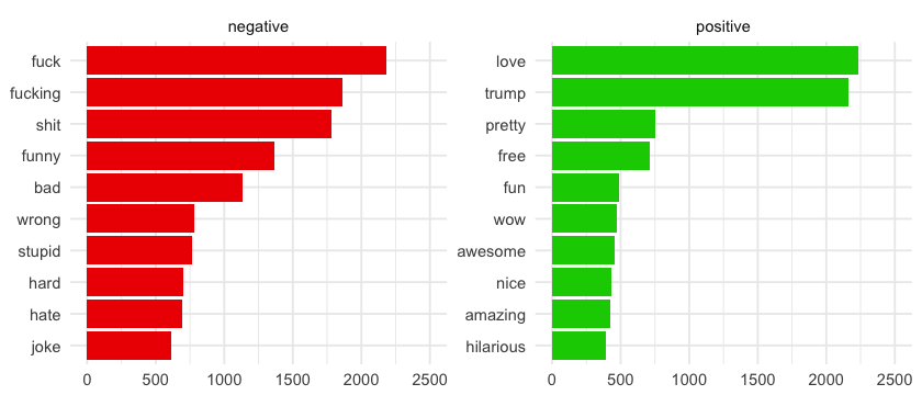
There is a lot of strong words here! And I'm pretty sure this trump positive word we are seeing is not quite the same Trump John has been talking about non stop for the last two years… and not precisely in a positive way… I could include this word in a custom_stop_words dataframe, but I'm going leave it like that for now.

Also… not sure why funny is in the negative category 🤔 I know it can be used as weird or something like that, but I think this happens because I'm not a native English speaker 🤷🏻 ♀️

Are there more positive or negative words?

tidy_yt_comments %>%
  inner_join(get_sentiments("bing"), by = "word") %>% 
  count(word, sentiment, sort = TRUE) %>% 
  group_by(sentiment) %>%
  top_n(10) %>%
  ungroup() %>%
  mutate(sentiment = reorder(sentiment, nn)) %>%
  ggplot(aes(sentiment, nn)) +
  geom_col(aes(fill = sentiment), show.legend = FALSE) +
  scale_fill_manual(values = c("green3", "red2")) +
  ylab(NULL) +
  xlab(NULL) +
  coord_flip() +
  theme_minimal()

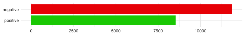
Definitely more negative than positive words. OK.

More sentiments in comments

There is a different lexicon, the nrc one, that classifies the words into more categories: two sentiments: positive and negative, and eight basic emotions: anger, anticipation, disgust, fear, joy, sadness, surprise, and trust. Let's check what we find!

tidy_yt_comments  %>%
  inner_join(get_sentiments("nrc"), by = "word") %>% 
  count(word, sentiment, sort = TRUE) %>% 
  group_by(sentiment) %>%
  top_n(10) %>%
  ungroup() %>%
  mutate(word = reorder(word, nn)) %>%
  ggplot(aes(word, nn, fill = sentiment)) +
  geom_col(show.legend = FALSE) +
  facet_wrap(~sentiment, scales = "free_y") +
  xlab(NULL) +
  ylab(NULL) +
  theme(axis.text.x = element_text(angle = 90, hjust = 1)) +
  coord_flip() +
  theme_minimal()

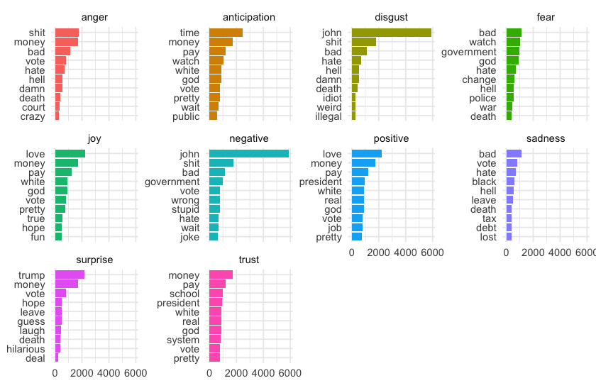
OK… a few comments here.

john is considered a negative word associated with disgust… So I checked and found that it means either a toilet or a prostitute's client, so now I get it 🚽 Either way, I'm going to include it in the custom_stop_words dataframe because it is a word so frequent that makes every other word disproportionate.
trump again is considered a positive word, associated with surprise (no doubt about the surprise element for both the word and the character though).

custom_stop_words <- bind_rows(data_frame(word = c("john"), 
                                          lexicon = c("custom")),
                               stop_words)

yt_comments %>%
  tidytext::unnest_tokens(word, com_text) %>%
  anti_join(custom_stop_words, by = "word") %>%
  inner_join(get_sentiments("nrc"), by = "word") %>% 
  count(word, sentiment, sort = TRUE) %>% 
  group_by(sentiment) %>%
  top_n(10) %>%
  ungroup() %>%
  mutate(word = reorder(word, nn)) %>%
  ggplot(aes(word, nn, fill = sentiment)) +
  geom_col(show.legend = FALSE) +
  facet_wrap(~sentiment, scales = "free_y") +
  scale_y_continuous(breaks = c(0, 1000, 2000)) +
  xlab(NULL) +
  ylab(NULL) +
  theme(axis.text.x = element_text(angle = 90, hjust = 1)) +
  coord_flip() +
  theme_minimal()

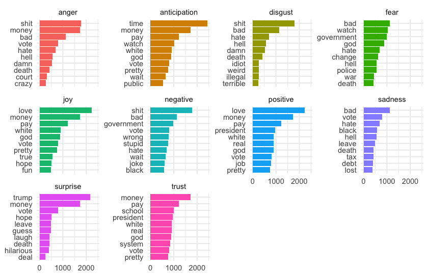
There are very controversial classifications on this nrc lexicon, especially with the terms black, classified as negative (and sadness) and white as positive (and joy, anticipation and trust). I don't like this at all…

I also have some comments:

goverment is negative while president is positive. Just caught my attention.
money: 💰 what is wrong with this word?! Apparently it is a very confusing one, because it is linked with positive sentiment and anticipation, joy, surprise and trust emotions, but also with anger 🤔

Anyway, these are side comments because they are about the lexicon (or the human nature!) and not this analysis. Bottom line: I don't like this lexicon 😒

What is the most present sentiment/emotion?

yt_comments %>%
  tidytext::unnest_tokens(word, com_text) %>%
  anti_join(custom_stop_words, by = "word") %>%
  inner_join(get_sentiments("nrc"), by = "word") %>% 
  count(word, sentiment, sort = TRUE) %>% 
  group_by(sentiment) %>%
  top_n(10) %>%
  ungroup() %>%
  mutate(pos_neg = ifelse(sentiment %in% c("positive", "anticipation", "joy", "trust", "surprise"), 
                          "Positive", "Negative")) %>%
  ggplot(aes(reorder(sentiment, nn), nn)) +
  geom_col(aes(fill = pos_neg), show.legend = FALSE) +
  scale_fill_manual(values = c("red2", "green3")) +
  xlab(NULL) +
  ylab(NULL) +
  coord_flip()

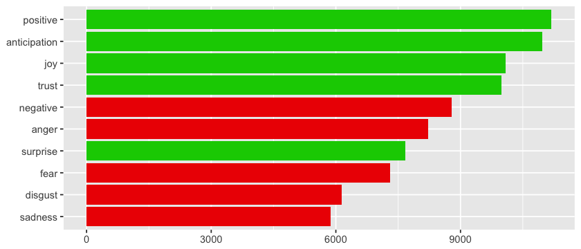
According to this lexicon, there are more positive than negative words! The opposite of what we found using the bing lexicon. The thing about this one is that allows us to analyze other sentiments as well. But of course I'm not going to use it anymore 😤

Most used n-grams

Other interesting thing to do is find the most common n-grams (threads of n amount of words that tend to co-occur).

yt_comments %>%
  tidytext::unnest_tokens(five_gram, com_text, token = "ngrams", n = 5) %>%
  count(five_gram, sort = TRUE) %>%
  top_n(10) %>%
  mutate(five_gram = reorder(five_gram, nn)) %>%
  ggplot(aes(five_gram, nn)) +
  geom_col(fill = "red", show.legend = FALSE) +
  xlab(NULL) +
  ylab(NULL) +
  coord_flip() +
  theme_minimal()

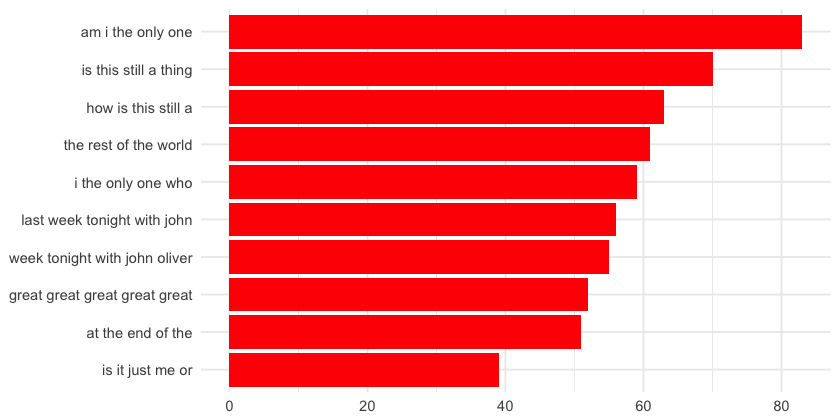
“how is this still a” and “is this still a thing” of course ring a bell for those of us who watch the show, since it has a section called “How is this still a thing?" questioning certain traditions or things that for some reason seemed adequate at some point in time, but now are totally absurd. Like voting for the US Presidential Elections on Tuesday, or the swimsuit issue of the Sports Illustrated magazine 🙄

The “am i the only one”, “i the only one who” and “is it just me or” 5-grams shows us how much people love rethorical questions! Like a lot! I'm going to take a peek at these comments!

am_i_the_only_one <- yt_comments %>%
  tidytext::unnest_tokens(five_gram, com_text, token = "ngrams", n = 5) %>%
  filter(five_gram == "am i the only one") %>%
  select(com_id)

datatable(head(yt_comments[yt_comments$com_id %in% am_i_the_only_one$com_id, c(7, 3)], 30), 
          rownames = FALSE,
          options = list(pageLength = 5)) %>% 
  formatStyle(c(1:2), `font-size` = '15px')

And a very strange 5-gram: “great great great great great”… I have to check what this is about!

great_great_great_great_great <- yt_comments %>%
  tidytext::unnest_tokens(five_gram, com_text, token = "ngrams", n = 5) %>%
  filter(five_gram == "great great great great great") %>%
  select(com_id) 

datatable(head(yt_comments[yt_comments$com_id %in% great_great_great_great_great$com_id, c(7, 3)], 1), 
          rownames = FALSE,
          options = list(pageLength = 5)) %>% 
  formatStyle(c(1:2), `font-size` = '15px')

Just like I suspected, this is one very long concatenation of the word “great”. This guy is a very, very enthusiastic atheist who is referring to a very old ancestor, so it doesn't count for this analysis.

Moving on…

Sentiment Analysis on comments

Similar to what I did for every word, now I join the words in the tidy_yt_comments dataset with the sentiment on the bing lexicon, and then count how many positive and negative words are in every comment. Then compute the sentiment as positive - negative, to finally join this to the yt_comment dataset.

library(tidyr) 

yt_comment_sent <- tidy_yt_comments  %>%
  inner_join(get_sentiments("bing"), by = "word") %>% 
  count(com_id, sentiment) %>%
  spread(sentiment, nn, fill = 0) %>%
  mutate(sentiment = positive - negative) %>% 
  ungroup() %>% 
  left_join(yt_comments, by = "com_id") %>% 
  arrange(sentiment)

The longer the comment, the higher potential for higher sentiment. Let's take a look at the extremes. The most negative comments according to the bing lexicon are:

datatable(head(yt_comment_sent[, c(10, 12, 6)], 30), 
          rownames = FALSE,
          options = list(pageLength = 1)) %>% 
  formatStyle(c(1:3), `font-size` = '15px')

And the most positive:

datatable(tail(yt_comment_sent[, c(10, 12, 6)], 30), 
          rownames = FALSE,
          options = list(pageLength = 1)) %>% 
  formatStyle(c(1:3), `font-size` = '15px')

See? People get passionate about the stories on this show 😮

Sentiment Analysis on videos

Let's see what we find when grouping the comments by video, and check for the most extreme ones.

yt_title_sent <- yt_comment_sent %>% 
  group_by(short_title, vid_created) %>% 
  summarise(pos           = sum(positive),
            neg           = sum(negative),
            sent_mean     = mean(sentiment),
            sentiment     = pos - neg) %>% 
  ungroup() %>% 
  arrange(-sentiment)
  
head(yt_title_sent, 7) %>% bind_rows(tail(yt_title_sent, 7)) %>% 
  ggplot(aes(reorder(short_title, sentiment), sentiment) ) +
  geom_col(aes(fill = sentiment > 0), show.legend = FALSE) +
  scale_fill_manual(values = c("red2", "green3")) +
  xlab(NULL) +
  ylab(NULL) +
  coord_flip() +
  theme_minimal()

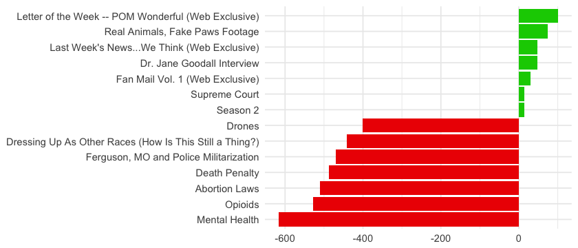The most positive videos are not actually main stories, but small stories or web specials. But the most negative ones are main stories about very hard topics like mental health, opioids and abortion, that makes people outraged. This totally makes sense: John always mixes hard stories with some comic relief in between. As he never covers a happy ending main story, the happy videos are some comic short ones or web exclusives.

You can check what are these episodes about below.

datatable(
  head(yt_title_sent, 7) %>% 
    bind_rows(tail(yt_title_sent, 7)) %>% 
    left_join(videos, by = "short_title") %>% 
    select(short_title, short_desc, sentiment),
  rownames = FALSE,
  options = list(pageLength = 7)) %>%
  formatStyle(c(1:3), `font-size` = '15px')

Youtube vs Facebook

My husband and I were discussing which audience would be more positive: the Youtube one or the Facebook one. We came up with the theory that Youtube seems more aggressive for some reason, but it was just our intuition. Now that I have the chance, I'm going to find out!

Fetching Facebook videos and comments

First I have to retrieve Facebook videos. I find the Rfacebook package way easier than tuber to interact with the Facebook Graph API, since you don't have to deal with pages to get the videos nor the comments.

You have to create a temporary access token (you can also try with a more permanent one, all you need to know is in this package documentation) and you are ready! With getPage and n = 5000 you retrieve 5000 posts. It is an exaggerated number, but I want to make sure I get all of them (there are 559 at the moment, in case you are wondering).

As I want only the videos coming from Youtube (so I can compare the comments), I filter the posts using a regular expression and then join the table with the videos dataframe from the Youtube videos to have the video information.

library(Rfacebook)

fb_token <- ####

fb_page <- getPage("LastWeekTonight", fb_token, n = 5000)

videos_fb <- fb_page %>% 
  filter(type == "video" &
           link == str_match(link, "^https://www.youtube.com/watch\\?v=.+")) %>% 
  mutate(ids = str_match(link, "^https://www.youtube.com/watch\\?v=([^&]+)")[,2]) %>% 
  left_join(videos, by = c("ids" = "id")) %>% 
  filter(!is.na(short_title))

Then I retrieve the comments.

library(purrr)
fb_com <- lapply(videos_fb$id, getPost, token = fb_token, n = 300)

fb_comments <- {}
for (i in 1:length(fb_com)) {
  post_id_fb   <- fb_com[[i]]$post$id
  com_id       <- fb_com[[i]]$comments$id
  com_text     <- fb_com[[i]]$comments$message
  com_created  <- fb_com[[i]]$comments$created_time
  fb_comments  <- fb_comments %>% 
    bind_rows(data.frame(post_id_fb, com_id, com_text, com_created))
}

To prepare the data for the comparison I used a lot of code, and very similar than the one used for Youtube! I don't want to get either repetitive or boring, so I'm not showing it here but you can see everything here.

I kept only 300 comments for every video on every platform.

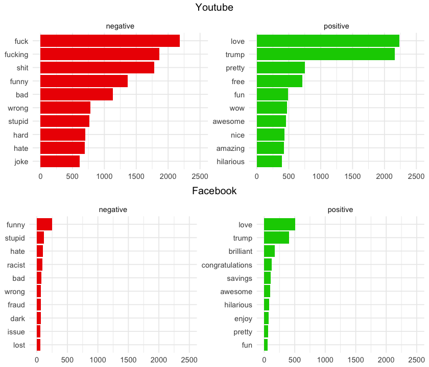
Youtube vs Facebook - Positive and Negative words

One thing I'm curious about is the difference in words used in both platforms. On (my) Facebook, people don't swear that much, probably because they are fiends with their grandmother… But let's put this theory to test, let's plot them together!

library(gridExtra)

grid.arrange(arrangeGrob(yt_pos_neg_words, top = "Youtube"), 
             arrangeGrob(fb_pos_neg_words, top = "Facebook"), nrow = 2)

Some remarks here:

People don't talk as much on Facebook! Youtube's words exceed 2,000 and Facebook's ones only go up to 500. I thought people on Facebook would be more verbal than on Youtube, but I only use this platform to see some specific videos and I've never left (or even read!) a comment there, so I'm far from an expert on this field.
People don't use the F-word that much on Facebook! I attribute it the the granny effect 👵

Youtube vs Facebook - Sentiment on videos

To compare comments I filter only the videos in both platforms (this is part of what is shown here) and plot the sentiment chronologically (try to hover over the lines to see the date and name of the video). Here I use the mean of sentiment for every chapter.

library(plotly)
ggplotly(comments_by_title %>%
  
  ggplot(aes(x = reorder(short_title, vid_created), 
             text = paste(short_title, "<br />",  vid_created))) +
  geom_line(aes(y = mean_sent_fb, group = 1), color = "blue") +
  geom_line(aes(y = mean_sent_yt, group = 1), color = "red") +
  geom_hline(yintercept = 0) +
  xlab(NULL) +
  ylab(NULL) +
  theme_minimal() +
  theme(axis.text.x = element_blank()),
tooltip = "text")

So Facebook audience is more positive than the Youtube one for almost every video. Just as we thought 😎

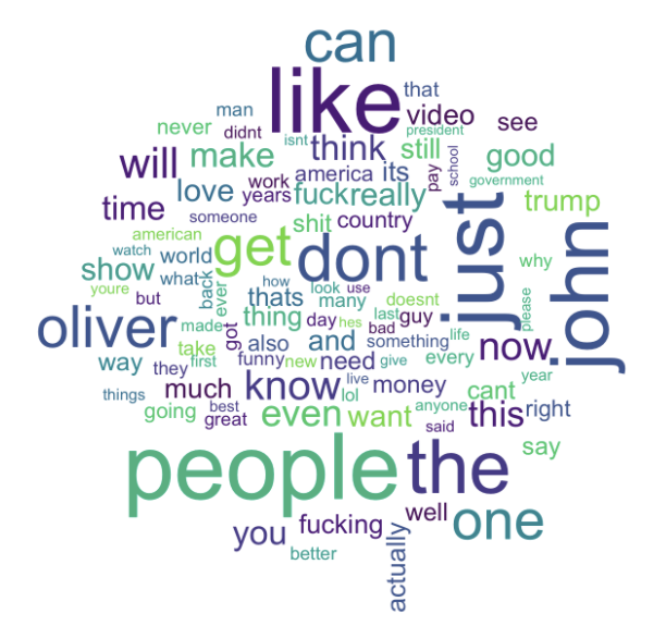
Wordcloud!

You were probably hoping for this! I couldn't pass up the opportunity to make a wordcloud 🎉 Are those awesome or what?!

library(wordcloud)
library(viridis)
library(tm)

words <- toString(yt_comments$com_text) %>%
  str_split(pattern = " ", simplify = TRUE)

wordcloud(words, colors = viridis::viridis_pal(end = 0.8)(10),
          min.freq = 800, random.color = TRUE, max.words = 100,
          scale = c(3.5,.03))

The end

Well, I hope you enjoyed this article as much as I did while writing it! It was so amusing to play with all these tools, and find out the feelings behind all those people who, like me, enjoy this show. If you haven't watch any episode yet, I recommend you give it a try. As we can see here: you won't probably be indifferent about it!

Despite this post being fairly extensive, it was actually hard for me to pick what to show here. You can find the complete analysis here, and feel free to reach out to me with your comments 😃